【第07讲】图论模型 返回首页
作者:欧新宇(Xinyu OU)
当前版本:Release v1.0
开发平台:Python3.11
运行环境:Intel Core i7-7700K CPU 4.2GHz, nVidia GeForce GTX 1080 Ti
本教案为非完整版教案,请结合课程PPT使用。
最后更新:2024年4月11日
一、NetworkX库简介
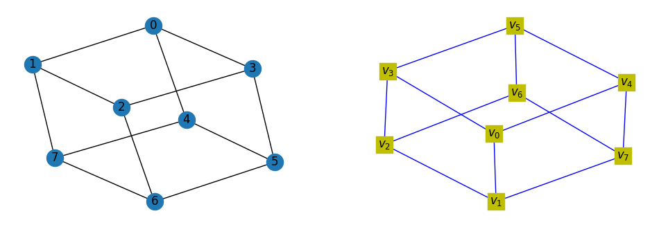
例1: 构造一个三正则图
# Lec0701_A_NetworkX_Example
import networkx as nx
import matplotlib.pyplot as plt

# 1. 绘制一个三正则图
# 1.1 构造三正则图
plt.figure(figsize=(12, 4))       # 定义画板的尺度
G = nx.cubical_graph()            # 生成一个3正则图
# 2. 使用NetworkX绘图
plt.subplot(121)                  # 激活1号子窗口
nx.draw(G, with_labels=True)      # 绘制图G,并附上图的标号

# 2. 为三正则图添加一些属性
plt.subplot(122)
s = ['$v_' + str(i) + '$' for i in range(8)]    # 添加顶点描述
s = dict(zip(range(8), s))                      # 构造顶点标注的字符字典{ID: Desc}
nx.draw(G, labels=s, node_color='y', node_shape='s', edge_color='b')  # 添加属性
plt.show()
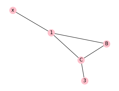
例2: 通过手工构造结点和边来创建图
# Lec0702_AddNodeEdge
import networkx as nx
import matplotlib.pyplot as plt

# 1. 定义图G的顶点和边
G = nx.Graph()
G.add_node('x')                  # 添加编号为x的一个顶点
G.add_nodes_from([1, 'B'])       # 从列表中添加多个顶点
G.add_edge(1, 'B')               # 添加顶点1和B之间的一条边
G.add_edge('x', 1, weight=0.5)   # 添加顶点x和1之间权重为0.5的一条边
e = [(1,'B',0.3), ('B','C',0.9), (1,'C',0.5), ('C',3,1.2)]   # 批量定义赋权边
G.add_weighted_edges_from(e)     # 从列表中添加多条赋权边

# 2. 输出图G
print(G.adj)                     # 显示图的邻接表的字典数据
plt.figure(figsize=(4, 3))       # 使用plt库定义图的尺度(可省略)
nx.draw(G, with_labels=True, node_color='pink')              # 绘制带顶点标签的图G
plt.show()
{'x': {1: {'weight': 0.5}},
   1: {'B': {'weight': 0.3}, 'x': {'weight': 0.5}, 'C': {'weight': 0.5}},
 'B': {1: {'weight': 0.3}, 'C': {'weight': 0.9}},
 'C': {'B': {'weight': 0.9}, 1: {'weight': 0.5}, 3: {'weight': 1.2}},
   3: {'C': {'weight': 1.2}}}
例3: 构造有向图
# Lec0703_DiGraph
import networkx as nx
import matplotlib.pyplot as plt

# 1. 定义图G的顶点和边
G = nx.DiGraph()                     # 初始化有向图
G.add_nodes_from(range(1, 7))        # 构造顶点标
List = [(1,2),(1,3),(2,3),(3,2),(3,5),(4,2),(4,6),(5,2),(5,4),(6,5),(1,6)]  # 定义边序列
G.add_edges_from(List)               # 构造有向边

# 2. 输出图
# 2.1 绘制图
pos = nx.shell_layout(G)             # 顶点在多个同心圆上分布
plt.figure(figsize=(4, 3))           # 使用plt库定义图的尺度(可省略)
nx.draw(G, pos, with_labels=True, font_weight='bold', node_color='y')   # 定义图的样式
plt.show()
# 2.2 输出图的邻接矩阵
print(G.adj)                                  # 输出图G的邻接矩阵字典
W = nx.to_numpy_array(G)                      # 输出图G的邻接矩阵
print('AdjacencyMatrix = \n {}'.format(W));
{1: {2: {}, 3: {}, 6: {}},
 2: {3: {}},
 3: {2: {},
 5: {}},
 4: {2: {}, 6: {}}, 5: {2: {}, 4: {}},
 6: {5: {}}}
AdjacencyMatrix =
 [[0. 1. 1. 0. 0. 1.]
 [0. 0. 1. 0. 0. 0.]
 [0. 1. 0. 0. 1. 0.]
 [0. 1. 0. 0. 0. 1.]
 [0. 1. 0. 1. 0. 0.]
 [0. 0. 0. 0. 1. 0.]]

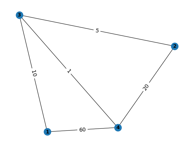
例4:加权图
# Lec0704_WeightedGraph
import networkx as nx
import matplotlib.pyplot as plt
import numpy as np

plt.figure(figsize=(4, 3))           # 使用plt库定义图的尺度(可省略)
G = nx.Graph()
List=[(1, 3, 10), (1, 4, 60), (2, 3, 5), (2, 4, 20), (3, 4, 1)]
G.add_nodes_from(range(1,5))
G.add_weighted_edges_from(List)
W1 = nx.to_numpy_array(G)                 # 从图G导出权重邻接矩阵
W2 = nx.get_edge_attributes(G, 'weight')  # 导出赋权边的字典数据
pos = nx.spring_layout(G)
nx.draw(G, pos, with_labels=True, font_weight='bold')
nx.draw_networkx_edge_labels(G, pos, font_size=13, edge_labels=W2)
print('邻接矩阵为:\n', W1)
print('邻接表字典为:\n', G.adj)
print('邻接表列表为:\n', list(G.adjacency()))
print('列表字典为:\n', nx.to_dict_of_lists(G))
np.savetxt('../../Data/Lec07/data0804.txt', W1, fmt='%d')  # 邻接矩阵保存到文本文件
plt.show()
邻接矩阵为:
 [[ 0.  0. 10. 60.]
 [ 0.  0.  5. 20.]
 [10.  5.  0.  1.]
 [60. 20.  1.  0.]]
邻接表字典为:
 {1: {3: {'weight': 10}, 4: {'weight': 60}}, 2: {3: {'weight': 5}, 4: {'weight': 20}}, 3: {1: {'weight': 10}, 2: {'weight': 5}, 4: {'weight': 1}}, 4: {1: {'weight': 60}, 2: {'weight': 20}, 3: {'weight': 1}}}
邻接表列表为:
 [(1, {3: {'weight': 10}, 4: {'weight': 60}}), (2, {3: {'weight': 5}, 4: {'weight': 20}}), (3, {1: {'weight': 10}, 2: {'weight': 5}, 4: {'weight': 1}}), (4, {1: {'weight': 60}, 2: {'weight': 20}, 3: {'weight': 1}})]
列表字典为:
 {1: [3, 4], 2: [3, 4], 3: [1, 2, 4], 4: [1, 2, 3]}
二、最短路径问题
例5:最小旅行费用问题
# Lec0705_Dijkstra_MinimumTravelFee0607
import networkx as nx

G = nx.DiGraph()
List = [(1,2,6), (1,3,3), (1,4,1), (2,5,1), (3,2,2), (3,4,2), (4,6,10), (5,4,6),
        (5,6,4), (5,7,3), (5,8,6), (6,5,10), (6,7,2), (7,8,4), (9,5,2), (9,8,3)]
G.add_nodes_from(range(1,10))
G.add_weighted_edges_from(List)
path = nx.dijkstra_path(G, 1, 8, weight='weight')       # 求最短路径
d = nx.dijkstra_path_length(G, 1, 8, weight='weight')   # 求最短路径费用(权重)
print('最短路径为:', path)
print('最小费用为:', d)
最短路径为: [1, 3, 2, 5, 8]
最小费用为: 12
例6:求图中的赋权图所有顶点之间的最短距离矩阵和最短路径
# Lec0706_Flord0608
import networkx as nx
import numpy as np

G = nx.Graph()
List = [(1, 3, 10), (1, 4, 60), (2, 3, 5), (2, 4, 20), (3, 4, 1)]
G.add_nodes_from(range(1,5))
G.add_weighted_edges_from(List)
d = nx.floyd_warshall_numpy(G)
print('最短距离矩阵为:\n', d)
path = nx.shortest_path(G, weight='weight', method='bellman-ford')
for i in range(1,len(d)):
    for j in range(i+1, len(d)+1):
        print('顶点{}到顶点{}的最短路径为:'.format(i,j), path[i][j])
最短距离矩阵为:
 [[ 0. 15. 10. 11.]
 [15.  0.  5.  6.]
 [10.  5.  0.  1.]
 [11.  6.  1.  0.]]
顶点1到顶点2的最短路径为: [1, 3, 2]
顶点1到顶点3的最短路径为: [1, 3]
顶点1到顶点4的最短路径为: [1, 3, 4]
顶点2到顶点3的最短路径为: [2, 3]
顶点2到顶点4的最短路径为: [2, 3, 4]
顶点3到顶点4的最短路径为: [3, 4]
例7:设备更新问题
# Lec0707_DeviceUpdate0609
import numpy as np
import networkx as nx
import pylab as plt

a=np.zeros((6,6))
a[0,1:]=[15,20,27,37,54]
a[1,2:]=[15,20,27,37]; a[2,3:]=[16,21,28];
a[3,4:]=[16,21]; a[4,5]=17
G = nx.DiGraph(a)  #构造赋权有向图,顶点编号为0,1,…,5
p = nx.shortest_path(G,0,5,weight='weight')
d = nx.shortest_path_length(G,0,5,weight='weight')
print('path=',p); print('d=',d)

plt.rc('font',size=16)
pos = nx.shell_layout(G)  #设置布局
w = nx.get_edge_attributes(G,'weight')
key = range(6)
s = ['v'+str(i+1) for i in key]
s = dict(zip(key,s)) #构造用于顶点标注的字符字典
nx.draw(G, pos, font_weight='bold', labels=s, node_color='r')
nx.draw_networkx_edge_labels(G, pos, edge_labels=w)
path_edges = list(zip(p, p[1:]))
nx.draw_networkx_edges(G, pos, edgelist=path_edges,
            edge_color='r', width=3)
plt.savefig('../../Data/Lec07/fig6_9.png', dpi=500)
plt.show()
path= [0, 2, 5]
d= 48.0

例8:仓库选址问题
# Lec0708_AddressSelection0610
import numpy as np
import networkx as nx

L=[(1,2,20), (1,5,15), (2,3,20), (2,4,60), (2,5,25), (3,4,30), (3,5,18), (5,6,15)]
G = nx.Graph(); G.add_nodes_from(np.arange(1,7))
G.add_weighted_edges_from(L)
d = nx.floyd_warshall_numpy(G)
d = np.array(d)  #转换为array数组
md = np.max(d, axis=1)   #逐行求最大值
mmd = min(md)          #求最小值
ind = np.argmin(md)+1     #求最小值的地址
print(d); print("最小值为:", mmd)
print("最小值的地址为:", ind)
[[ 0. 20. 33. 63. 15. 30.]
 [20.  0. 20. 50. 25. 40.]
 [33. 20.  0. 30. 18. 33.]
 [63. 50. 30.  0. 48. 63.]
 [15. 25. 18. 48.  0. 15.]
 [30. 40. 33. 63. 15.  0.]]
最小值为: 33.0
最小值的地址为: 3
三、最小生成树
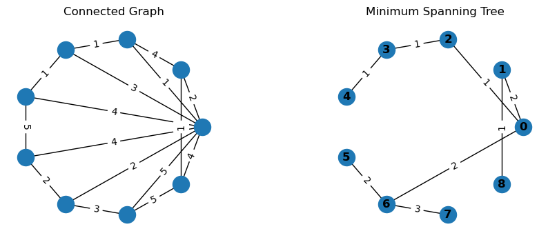
例9:自然村架设通讯线路
# Lec0709_SpanningTree0612
import networkx as nx
import pylab as plt

L = [(0,1,2),(0,2,1),(0,3,3),(0,4,4),(0,5,4),(0,6,2),(0,7,5),(0,8,4),(1,2,4),(1,8,1),(2,3,1),(3,4,1),(4,5,5),(5,6,2),(6,7,3),(7,8,5)]
G = nx.Graph()
G.add_weighted_edges_from(L)
T = nx.minimum_spanning_tree(G)   # 返回可迭代对象
c = nx.to_numpy_array(T)          # 返回最小生成树的邻接矩阵
print("邻接矩阵 AdjMatrix = \n",c)
w = c.sum()/2                     #求最小生成树的权重
print("最小生成树的权重 W =",w)

plt.figure(figsize=(10, 4))
pos = nx.circular_layout(G)
plt.subplot(121)  # 绘制连通图
plt.title('Connected Graph', fontsize=12)
nx.draw(G,pos)
w1 = nx.get_edge_attributes(G, 'weight')
nx.draw_networkx_edge_labels(G, pos, edge_labels=w1)

plt.subplot(122)  #绘制最小生成树
plt.title('Minimum Spanning Tree', fontsize=12)
nx.draw(T, pos, with_labels=True, font_weight='bold')
w2 = nx.get_edge_attributes(T, 'weight')
nx.draw_networkx_edge_labels(T, pos, edge_labels=w2)
plt.subplots_adjust(wspace=0.5)
plt.show()
邻接矩阵 AdjMatrix =
 [[0. 2. 1. 0. 0. 0. 2. 0. 0.]
 [2. 0. 0. 0. 0. 0. 0. 0. 1.]
 [1. 0. 0. 1. 0. 0. 0. 0. 0.]
 [0. 0. 1. 0. 1. 0. 0. 0. 0.]
 [0. 0. 0. 1. 0. 0. 0. 0. 0.]
 [0. 0. 0. 0. 0. 0. 2. 0. 0.]
 [2. 0. 0. 0. 0. 2. 0. 3. 0.]
 [0. 0. 0. 0. 0. 0. 3. 0. 0.]
 [0. 1. 0. 0. 0. 0. 0. 0. 0.]]
最小生成树的权重 W = 13.0
四、最大流与最小费用流问题
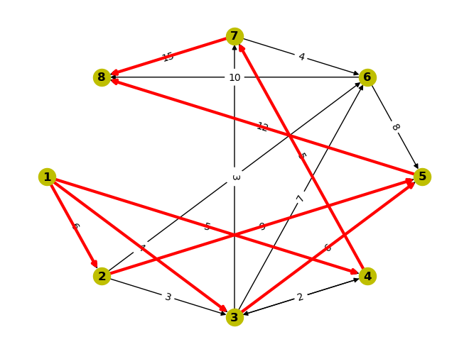
例10:求图中1到8的最大流
# Lec0710_MaximumFlow0617
import numpy as np
import networkx as nx
import pylab as plt

L = [(1,2,6),(1,3,4),(1,4,5),(2,3,3),(2,5,9),(2,6,9),
    (3,4,5),(3,5,6),(3,6,7),(3,7,3),(4,3,2),(4,7,5),
    (5,8,12),(6,5,8),(6,8,10),(7,6,4),(7,8,15)]
G = nx.DiGraph()
G.add_nodes_from(range(1,9))
G.add_weighted_edges_from(L,weight='capacity')

value, flow_dict = nx.maximum_flow(G, 1, 8)
print("最大流的流量为:",value)
print("最大流为:", flow_dict)

n = len(flow_dict)
adj_mat = np.zeros((n, n), dtype=int)
for i, adj in flow_dict.items():
    for j, weight in adj.items():
        adj_mat[i-1,j-1] = weight
print("最大流的邻接矩阵为:\n",adj_mat)
ni, nj = np.nonzero(adj_mat)  #非零弧的两端点编号
plt.rc('font', size=16)
pos = nx.shell_layout(G)  #设置布局
w = nx.get_edge_attributes(G,'capacity')
nx.draw(G,pos,font_weight='bold', with_labels=True, node_color='y')
nx.draw_networkx_edge_labels(G, pos, edge_labels=w)
path_edges = list(zip(ni+1, nj+1))
nx.draw_networkx_edges(G,pos, edgelist=path_edges, edge_color='r', width=3)
plt.show()
最大流的流量为: 15
最大流为:
{1: {2: 6, 3: 4, 4: 5},
 2: {3: 0, 5: 6, 6: 0},
 3: {4: 0, 5: 4, 6: 0, 7: 0},
 4: {3: 0, 7: 5},
 5: {8: 10},
 6: {5: 0, 8: 0},
 7: {6: 0, 8: 5},
 8: {}}
最大流的邻接矩阵为:
 [[ 0  6  4  5  0  0  0  0]
 [ 0  0  0  0  6  0  0  0]
 [ 0  0  0  0  4  0  0  0]
 [ 0  0  0  0  0  0  5  0]
 [ 0  0  0  0  0  0  0 10]
 [ 0  0  0  0  0  0  0  0]
 [ 0  0  0  0  0  0  0  5]
 [ 0  0  0  0  0  0  0  0]]
例11:基于最大流的招聘问题
- 解一
# Lec0711 EmploymentMaximumFlow0618
import numpy as np
import networkx as nx
node=['s','A','B','C','D','E','2b','3b','4b','1','2','3','4','t']
n = len(node); G = nx.DiGraph(); G.add_nodes_from(node)
L = [('s','A',4),('s','B',3),('s','C',3),('s','D',2),('s','E',4),('A','2b',1),
    ('A','1',1),('A','3b',1),('A','4b',1),('B','2b',1),('B','1',1),('B','3',1),
    ('B','4b',1),('C','1',1),('C','2',1),('C','3',1),('C','4b',1),('D','1',1),
    ('D','2',1),('D','3b',1),('D','4b',1),('E','2b',1),('E','1',1),('E','3',1),
    ('E','4',1),('2b','2',2),('3b','3',1),('4b','4',2),('1','t',5),('2','t',4),
    ('3','t',4),('4','t',3)]

for k in range(len(L)):
    G.add_edge(L[k][0], L[k][1], capacity=L[k][2])
value, flow_dict = nx.maximum_flow(G, 's', 't')
print(value);
print(flow_dict)
A = np.zeros((n,n),dtype=int)
for i, adj in flow_dict.items():
    for j, f in adj.items():
        A[node.index(i), node.index(j)] = f
print(A)
16
{'s': {'A': 4, 'B': 3, 'C': 3, 'D': 2, 'E': 4}, 'A': {'2b': 1, '1': 1, '3b': 1, '4b': 1}, 'B': {'2b': 0, '1': 1, '3': 1, '4b': 1}, 'C': {'1': 1, '2': 1, '3': 1, '4b': 0}, 'D': {'1': 1, '2': 1, '3b': 0, '4b': 0}, 'E': {'2b': 1, '1': 1, '3': 1, '4': 1}, '2b': {'2': 2}, '3b': {'3': 1}, '4b': {'4': 2}, '1': {'t': 5}, '2': {'t': 4}, '3': {'t': 4}, '4': {'t': 3}, 't': {}}
[[0 4 3 3 2 4 0 0 0 0 0 0 0 0]
 [0 0 0 0 0 0 1 1 1 1 0 0 0 0]
 [0 0 0 0 0 0 0 0 1 1 0 1 0 0]
 [0 0 0 0 0 0 0 0 0 1 1 1 0 0]
 [0 0 0 0 0 0 0 0 0 1 1 0 0 0]
 [0 0 0 0 0 0 1 0 0 1 0 1 1 0]
 [0 0 0 0 0 0 0 0 0 0 2 0 0 0]
 [0 0 0 0 0 0 0 0 0 0 0 1 0 0]
 [0 0 0 0 0 0 0 0 0 0 0 0 2 0]
 [0 0 0 0 0 0 0 0 0 0 0 0 0 5]
 [0 0 0 0 0 0 0 0 0 0 0 0 0 4]
 [0 0 0 0 0 0 0 0 0 0 0 0 0 4]
 [0 0 0 0 0 0 0 0 0 0 0 0 0 3]
 [0 0 0 0 0 0 0 0 0 0 0 0 0 0]]
- 解二
# Lec0711-2 EmploymentMaximumFlow0618-2
import numpy as np
import cvxpy as cp
a = np.array([4, 3, 3, 2, 4])
x = cp.Variable((4,5), integer=True)
obj = cp.Maximize(cp.sum(x))
con = [cp.sum(x, axis=0) <= a,
        x[1,0]+x[1,1]+x[1,4] <= 2,
        x[2,0]+x[2,3] <= 1,
        sum(x[3,:-1]) <= 2, x>=0, x<=1]
prob = cp.Problem(obj, con)
prob.solve(solver='GLPK_MI')
print("最优值为:", prob.value)
print("最优解为:\n", x.value)
最优值为: 16.0
最优解为:
 [[1. 1. 1. 1. 1.]
 [1. 0. 1. 1. 1.]
 [1. 1. 1. 0. 1.]
 [1. 1. 0. 0. 1.]]
例12:最小费用问题
# Lec0712-3 FeeMaximnumFlow0619
import numpy as np
import networkx as nx
L = [('vs','v2',5,3),('vs','v3',3,6),('v2','v4',2,8),('v3','v2',1,2),('v3','v5',4,2),
    ('v4','v3',1,1),('v4','v5',3,4),('v4','vt',2,10),('v5','vt',5,2)]
G = nx.DiGraph()
for k in range(len(L)):
    G.add_edge(L[k][0], L[k][1], capacity=L[k][2], weight=L[k][3])
maxFlow = nx.max_flow_min_cost(G,'vs','vt')
print("所求最大流为:", maxFlow)
mincost = nx.cost_of_flow(G, maxFlow)
print("最小费用为:", mincost)

node = list(G.nodes())  # 导出顶点列表
n = len(node); flow_mat = np.zeros((n,n))
for i,adj in maxFlow.items():
    for j,f in adj.items():
        flow_mat[node.index(i), node.index(j)] = f
print("最大流的流量为:", sum(flow_mat[:,-1]))
print("最小费用最大流的邻接矩阵为:\n", flow_mat)
所求最大流为: {'vs': {'v2': 2, 'v3': 3}, 'v2': {'v4': 2}, 'v3': {'v2': 0, 'v5': 4}, 'v4': {'v3': 1, 'v5': 1, 'vt': 0}, 'v5': {'vt': 5}, 'vt': {}}
最小费用为: 63
最大流的流量为: 5.0
最小费用最大流的邻接矩阵为:
 [[0. 2. 3. 0. 0. 0.]
 [0. 0. 0. 2. 0. 0.]
 [0. 0. 0. 0. 4. 0.]
 [0. 0. 1. 0. 1. 0.]
 [0. 0. 0. 0. 0. 5.]
 [0. 0. 0. 0. 0. 0.]]
五、关键路径
例6.20 工程的关键路径
某项目工程由11项作业组成(分别用代号表示),其计划完成时间及活动间相互关系如下表所示,求活动的关键路径。
# Lec0713: CriticalPath0620
import cvxpy as cp

x = cp.Variable(8, pos=True)
L = [(1,2,5), (1,3,10), (1,4,11), (2,5,4), (3,4,4), (3,5,0), (4,6,15),
    (5,6,21), (5,7,25), (5,8,35), (6,7,0), (6,8,20), (7,8,15)]
obj = cp.Minimize(sum(x));
con = []
for k in range(len(L)):
    con.append(x[L[k][1]-1] >= x[L[k][0]-1] + L[k][2])
prob = cp.Problem(obj, con)
prob.solve(solver='GLPK_MI')
print('最优值为:', prob.value);
print('最优解为:', x.value)
最优值为: 156.0
最优解为: [ 0.  5. 10. 14. 10. 31. 35. 51.]
例6.21(续例6.20)
求例6.20中每个作业的最早开工时间、最迟开工时间和作业的关键路径。
# Lec0714: CriticalPath0621
import numpy as np
import cvxpy as cp

n =8; x = cp.Variable(n, pos=True); z = np.zeros(n)
L = [(1,2,5), (1,3,10), (1,4,11), (2,5,4), (3,4,4), (3,5,0), (4,6,15),
    (5,6,21), (5,7,25), (5,8,35), (6,7,0), (6,8,20), (7,8,15)]
obj = cp.Minimize(sum(x)); con = []
for k in range(len(L)):
    con.append(x[L[k][1]-1] >= x[L[k][0]-1] + L[k][2])
prob = cp.Problem(obj, con); prob.solve(solver='GLPK_MI')
print('最优值为', prob.value); print('最优解为:', x.value)
xx = x.value; z[-1] = xx[-1]
for k in range(n-1, 0, -1):
    z[k-1]=min([z[a[1]-1]-a[2] for a in L if a[0]==k])
print('z:', z); es=[]; lf=[]; ls=[]; ef=[]
for i in range(len(L)):
    es.append([L[i][0], L[i][1], xx[L[i][0]-1]])
    lf.append([L[i][0], L[i][1], z[L[i][1]-1]])
    ls.append([L[i][0], L[i][1], z[L[i][1]-1]-L[i][2]])
    ef.append([L[i][0], L[i][1], xx[L[i][0]-1]+L[i][2]])
print('作业最早开工时间如下:'); print(es)
print('作业最晚开工时间如下:'); print(ls)
最优值为 156.0
最优解为: [ 0.  5. 10. 14. 10. 31. 35. 51.]
z: [ 0.  6. 10. 16. 10. 31. 36. 51.]
作业最早开工时间如下:
[[1, 2, 0.0], [1, 3, 0.0], [1, 4, 0.0], [2, 5, 5.0], [3, 4, 10.0], [3, 5, 10.0], [4, 6, 14.0], [5, 6, 10.0], [5, 7, 10.0], [5, 8, 10.0], [6, 7, 31.0], [6, 8, 31.0], [7, 8, 35.0]]
作业最晚开工时间如下:
[[1, 2, 1.0], [1, 3, 0.0], [1, 4, 5.0], [2, 5, 6.0], [3, 4, 12.0], [3, 5, 10.0], [4, 6, 16.0], [5, 6, 10.0], [5, 7, 11.0], [5, 8, 16.0], [6, 7, 36.0], [6, 8, 31.0], [7, 8, 36.0]]
例6.22 用最长路的方法,求解例6.20。
# Lec0715: CriticalPath0622
import numpy as np
import cvxpy as cp

L = [(1,2,5), (1,3,10), (1,4,11), (2,5,4), (3,4,4), (3,5,0), (4,6,15),
    (5,6,21), (5,7,25), (5,8,35), (6,7,0), (6,8,20), (7,8,15)]
x = cp.Variable((8,8), integer=True); fun = 0
for i in range(len(L)):
    fun = fun + x[L[i][0]-1,L[i][1]-1] * L[i][2]
obj = cp.Maximize(fun); con =[ x>=0, x<=1]
out = [a[1]-1 for a in L if a[0]==1]  #起点相邻顶点的编号
con.append(sum(x[0,out])==1)   #起点发出弧的约束
ind = [a[0]-1 for a in L if a[1]==8]  #终点相邻顶点的编号
con.append(sum(x[ind,7])==1)   #终点进入弧的约束
for k in range(2,8):
    out = [a[1]-1 for a in L if a[0]==k]  #k的出弧的相邻顶点
    ind = [a[0]-1 for a in L if a[1]==k]  #k的入弧的相邻顶点
    con.append(sum(x[k-1,out])==sum(x[ind,k-1]))
prob = cp.Problem(obj, con); prob.solve(solver='GLPK_MI')
print('最优值为', prob.value); print('最优解为:\n', x.value)
ni, nj = np.nonzero(x.value)
print('关键路径的端点为:'); print(ni+1); print(nj+1)
最优值为 51.0
最优解为:
 [[0. 0. 1. 0. 0. 0. 0. 0.]
 [0. 0. 0. 0. 0. 0. 0. 0.]
 [0. 0. 0. 0. 1. 0. 0. 0.]
 [0. 0. 0. 0. 0. 0. 0. 0.]
 [0. 0. 0. 0. 0. 1. 0. 0.]
 [0. 0. 0. 0. 0. 0. 0. 1.]
 [0. 0. 0. 0. 0. 0. 0. 0.]
 [0. 0. 0. 0. 0. 0. 0. 0.]]
关键路径的端点为:
[1 3 5 6]
[3 5 6 8]
例6.23(关键路线与计划网络的优化)
假设例6.20中所列的工程要求在49天内完成。为提前完成工程,有些作业需要加快进度,缩短工期,而加快进度需要额外增加费用。表6.6列出例6.20中可缩短工期的所有作业和缩短一天工期额外增加的费用。现在的问题是,如何安排作业才能使额外增加的总费用最少。
# Lec0716: CriticalPath0623
import numpy as np
import cvxpy as cp
L = [(1,2,5,5,0), (1,3,10,8,700), (1,4,11,8,400), (2,5,4,3,450), (3,4,4,4,0),
    (3,5,0,0,0), (4,6,15,15,0), (5,6,21,16,600), (5,7,25,22,300),
    (5,8,35,30,500), (6,7,0,0,0), (6,8,20,16,500), (7,8,15,12,400)]
x = cp.Variable(8, pos=True)
y = cp.Variable((8,8), integer=True); fun = 0
for i in range(len(L)):
    fun = fun + y[L[i][0]-1,L[i][1]-1] * L[i][4]
obj = cp.Minimize(fun); con =[x[7]-x[0]<=49, y>=0]
for i in range(len(L)):
    con.append(x[L[i][1]-1]-x[L[i][0]-1]+y[L[i][0]-1,L[i][1]-1]>=L[i][2])
    con.append(y[L[i][0]-1,L[i][1]-1]<=L[i][2]-L[i][3])
prob = cp.Problem(obj, con); prob.solve(solver='GLPK_MI')
print('最优值为', prob.value); print('x的取值为:\n', x.value)
print('y的取值为:\n', y.value); ni, nj = np.nonzero(y.value)
print('压缩工期的作业为:'); print(ni+1); print(nj+1)
最优值为 1200.0
x的取值为:
 [ 0.  5.  9. 13.  9. 30. 34. 49.]
y的取值为:
 [[0. 0. 1. 0. 0. 0. 0. 0.]
 [0. 0. 0. 0. 0. 0. 0. 0.]
 [0. 0. 0. 0. 0. 0. 0. 0.]
 [0. 0. 0. 0. 0. 0. 0. 0.]
 [0. 0. 0. 0. 0. 0. 0. 0.]
 [0. 0. 0. 0. 0. 0. 0. 1.]
 [0. 0. 0. 0. 0. 0. 0. 0.]
 [0. 0. 0. 0. 0. 0. 0. 0.]]
压缩工期的作业为:
[1 6]
[3 8]
例6. 24(续例6.23)最早开工时间和最迟开工时间
用Python求解例6.23,并求出相应的关键路径、各作业的最早开工时间和最迟开工时间。(如需要知道压缩工期后的关键路径,则需要稍复杂一点的计算。)
# Lec0717: CriticalPath0624
import numpy as np
import cvxpy as cp

L = [(1,2,5,5,0), (1,3,10,8,700), (1,4,11,8,400), (2,5,4,3,450), (3,4,4,4,0),
    (3,5,0,0,0), (4,6,15,15,0), (5,6,21,16,600), (5,7,25,22,300),
    (5,8,35,30,500), (6,7,0,0,0), (6,8,20,16,500), (7,8,15,12,400)]
n=8; x = cp.Variable(n, pos=True)
y = cp.Variable((n,n), integer=True); fun = 0
for i in range(len(L)):
    fun = fun + y[L[i][0]-1,L[i][1]-1] * L[i][4]
obj = cp.Minimize(fun+sum(x)); con =[x[7]-x[0]<=49, y>=0]

for i in range(len(L)):
    con.append(x[L[i][1]-1]-x[L[i][0]-1]+y[L[i][0]-1,L[i][1]-1]>=L[i][2])
    con.append(y[L[i][0]-1,L[i][1]-1]<=L[i][2]-L[i][3])
prob = cp.Problem(obj, con); prob.solve(solver='GLPK_MI')
print('最优值为', prob.value); print('x的取值为:\n', x.value)
print('y的取值为:\n', y.value); xx=x.value
yy = y.value; z = np.zeros(n); z[-1] = xx[-1]
for k in range(n-1, 0, -1):
    z[k-1] = min([z[a[1]-1]-a[2]+yy[a[0]-1,a[1]-1] for a in L if a[0]==k])
es = []; ls = []
for i in range(len(L)):
    es.append([L[i][0], L[i][1], xx[L[i][0]-1]])
    ls.append([L[i][0], L[i][1], z[L[i][1]-1]-L[i][2]+yy[L[i][0]-1,L[i][1]-1]])
print('es = {}'.format(es))
print('ls = {}'.format(ls))
最优值为 1349.0
x的取值为:
 [ 0.  5.  9. 13.  9. 30. 34. 49.]
y的取值为:
 [[0. 0. 1. 0. 0. 0. 0. 0.]
 [0. 0. 0. 0. 0. 0. 0. 0.]
 [0. 0. 0. 0. 0. 0. 0. 0.]
 [0. 0. 0. 0. 0. 0. 0. 0.]
 [0. 0. 0. 0. 0. 0. 0. 0.]
 [0. 0. 0. 0. 0. 0. 0. 1.]
 [0. 0. 0. 0. 0. 0. 0. 0.]
 [0. 0. 0. 0. 0. 0. 0. 0.]]
es = [[1, 2, 0.0], [1, 3, 0.0], [1, 4, 0.0], [2, 5, 5.0], [3, 4, 9.0], [3, 5, 9.0], [4, 6, 13.0], [5, 6, 9.0], [5, 7, 9.0], [5, 8, 9.0], [6, 7, 30.0], [6, 8, 30.0], [7, 8, 34.0]]
ls = [[1, 2, 0.0], [1, 3, 0.0], [1, 4, 4.0], [2, 5, 5.0], [3, 4, 11.0], [3, 5, 9.0], [4, 6, 15.0], [5, 6, 9.0], [5, 7, 9.0], [5, 8, 14.0], [6, 7, 34.0], [6, 8, 30.0], [7, 8, 34.0]]
例6.25 规定时间内完成作业的概率
已知例6.20中各项作业完成的三个估计时间如表6.8所示。如果规定时间为52天,求在规定时间内完成全部作业的概率。进一步,如果完成全部作业的概率大于等于95%,那么工期至少需要多少天?
# Lec0718: CriticalPath0625
import numpy as np
import cvxpy as cp
from scipy.stats import norm

L = np.array([(1,2,3,5,7),(1,3,8,9,16),(1,4,8,11,14),(2,5,3,4,5),
    (3,4,2,4,6),(3,5,0,0,0),(4,6,8,16,18),(5,6,18,20,28),(5,7,18,25,32),
    (5,8,26,33,52),(6,7,0,0,0),(6,8,11,21,25),(7,8,12,15,18)])
et = (L[:,2]+4*L[:,3]+L[:,4])/6  #计算均值
dt = (L[:,4]-L[:,2])**2/36       #计算方差
n = 8; x = cp.Variable((n,n), integer=True)
m = len(L); fun = 0

for i in range(m):
    fun=fun+x[L[i][0]-1,L[i][1]-1]*et[i]
obj = cp.Maximize(fun); con=[x>=0, x<=1]
out = np.where(L[:,0]==1)[0]  #起点的相邻顶点
con.append(cp.sum(x[0,L[out,1]-1])==1)
for k in range(2,n):
    out = np.where(L[:,0]==k)[0]  #顶点k发出弧的顶点
    ind = np.where(L[:,1]==k)[0]  #顶点k进入弧的顶点
    con.append(cp.sum(x[L[ind,0]-1,k-1]) == cp.sum(x[k-1,L[out,1]-1]))
ind = np.where(L[:,1]==n)  #终点的相邻顶点
con.append(cp.sum(x[L[ind,0]-1,n-1])==1)
prob = cp.Problem(obj, con); prob.solve(solver='GLPK_MI')
print('最优值为:', prob.value); print('最优解为:\n', x.value)
f = prob.value; xx = x.value; s2=0  #方差的初值

for i in range(m):
    s2 = s2 + xx[L[i][0]-1, L[i][1]-1]*dt[i]
s = np.sqrt(s2)
p = norm.cdf(52, f, s)  #计算标准差和概率
N = norm.ppf(0.95)*s+f; print('标准差s:', s)
print('概率p:', p); print('需要天数N:', N)
最优值为: 51.0
最优解为:
 [[0. 0. 1. 0. 0. 0. 0. 0.]
 [0. 0. 0. 0. 0. 0. 0. 0.]
 [0. 0. 0. 0. 1. 0. 0. 0.]
 [0. 0. 0. 0. 0. 0. 0. 0.]
 [0. 0. 0. 0. 0. 1. 0. 0.]
 [0. 0. 0. 0. 0. 0. 0. 1.]
 [0. 0. 0. 0. 0. 0. 0. 0.]
 [0. 0. 0. 0. 0. 0. 0. 0.]]
标准差s: 3.1622776601683795
概率p: 0.6240851829770754
需要天数N: 56.201483878755575
六、钢管订购和运输
本案例的详细教案请访问 Project08钢管订购和运输