【第04讲】微分方程的求解返回首页

作者：欧新宇（Xinyu OU）
当前版本：Release v1.0
开发平台：Python3.11
运行环境：Intel Core i7-7700K CPU 4.2GHz, nVidia GeForce GTX 1080 Ti
本教案为非完整版教案，请结合课程PPT使用。

最后更新：2024年3月19日

一、微分方程

例8.3 求解微分方程 $y' = -2y + 2x^2 + 2x, y(0) = 1$

# Lec0401: 例8.3 微分方程求解
import sympy as sp

x = sp.var('x')                                 # 定义符号型自变量
y = sp.Function('y')                            # 定义符号函数
eq = y(x).diff(x) + 2*y(x) - 2*x**2 - 2*x       # 定义微分方程
res = sp.dsolve(eq, ics = {y(0):1})             # 求解符号解
res = sp.simplify(res)                          # 对解方程进行化简
res

$y(x) = x^2 + e^{-2x}$

例8.4 求解二阶线性微分方程 $y'' - 2y' + y = e^x, y(0) = 1, y'(0) = -1$

# Lec0402: 例8.4 二阶线性微分方程
import sympy as sp

x = sp.var('x')
y = sp.Function('y')
eq = y(x).diff(x, 2) - 2*y(x).diff(x) + y(x) - sp.exp(x)
con = {y(0):1, y(x).diff(x).subs(x, 0):-1}
res = sp.dsolve(eq, ics = con)
res

$y(x) = (x(\frac{x}{2} - 2) + 1) e^x$

例8.5 已知输入信号为 $u(t) = e^{-t} cos(t)$ ，试求下面微分方程的解

$y^{(4)}(t) + 10y^{(3)}(t) + 35y''(t) + 50y'(t) + 24y(t) = u''(t), y(0)=0, y'(0)=-1, y''(0)=1, y'''(0)=1$

# Lec0403: 例8.5 三阶线性微分方程
import sympy as sp

t = sp.var('t')
y = sp.Function('y')
u = sp.exp(-t)*sp.cos(t)
eq = y(t).diff(t, 4) + 10*y(t).diff(t, 3) + 35*y(t).diff(t, 2) + 50*y(t).diff(t) + 24*y(t) - u.diff(t, 2)
con = {y(0):0, y(t).diff(t).subs(t, 0):-1, y(t).diff(t, 2).subs(t, 0):1, y(t).diff(t, 3).subs(t, 0):1}
res = sp.dsolve(eq, ics = con)
res = sp.expand(res)
res

$y(t) = -\frac{e^{-t} \sin(t)}{5} - \frac{7 e^{-t}}{3} + \frac{9e^{-2t}}{2} - \frac{14e^{-3t}}{5} + \frac{19e^{-4t}}{30}$

例8.6 求解微分方程组

试求： $\begin{cases} \frac{dx}{dt} = Ax \\\\ x(0) = [1, 1, 1]^T \end{cases}$ 的解，

其中 $x(t) = [x_1(t), x_2(t), x_3(t)]^T, A = \begin{bmatrix} 3 & -1 & 1 \\ 2 & 0 & -1 \\1 & -1 & 2 \end{bmatrix}.$

# Lec0404: 例8.6 求解微分方程组
import sympy as sp

t = sp.var('t')
x1, x2, x3 = sp.var('x1:4', cls = sp.Function)       # 定义符号函数
x = sp.Matrix([x1(t), x2(t), x3(t)])                 # 定义列向量
A = sp.Matrix([[3, -1, 1], [2, 0, -1], [1, -1, 2]])  # 定义系数矩阵
eq = x.diff(t) - A@x                                 # @ 表示矩阵乘法
res = sp.dsolve(eq, ics = {x1(0):1, x2(0):1, x3(0):1})
for i in range(0,3):
    print(res[i])
res[0]                                               # 使用Notebook渲染方程

Eq(x1(t), 4*exp(3*t)/3 - exp(2*t)/2 + 1/6)
Eq(x2(t), 2*exp(3*t)/3 - exp(2*t)/2 + 5/6)
Eq(x3(t), 2*exp(3*t)/3 + 1/3)

$x_1(t) = \frac{4e^{3t}}{3} - \frac{e^{2t}}{2} + \frac{1}{6}$

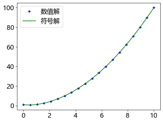
例8.7 求解微分方程 $y' = -2y + 2x^2 + 2x, y(0) = 1$ 的数值解，并分别画出数值解和符号解曲线

# Lec0405: 例8.7 常微分方程的数值解
import sympy as sp
import numpy as np
import matplotlib.pyplot as plt
from scipy.integrate import odeint
plt.rcParams['font.sans-serif'] = ['Microsoft YaHei']  # 使用微软雅黑字体显示标签

# 1. 计算方程数值解 (求数值解时，若为给出自变量范围，则手动设置自变量)
dy = lambda y, x: -2*y+2*x**2+2*x               # 自变量参数在函数参数最后
xt = np.linspace(0,10,20)                       # 自变量为0~10之间的20个数
yt = odeint(dy, 1, xt)                          # 求解数值解
plt.plot(xt, yt,'b*', label='数值解')           # 数值解曲线通常时离散的
print('x={}\n y={}'.format(xt, yt.flatten()))

# 2. 计算方程符号解
x = sp.var('x')                                 # 定义符号型自变量
y = sp.Function('y')                            # 定义符号函数
eq = y(x).diff(x) + 2*y(x) - 2*x**2 - 2*x       # 定义微分方程
res = sp.dsolve(eq, ics = {y(0):1})             # 求解符号解
resF = sp.lambdify(x, res.args[1], 'numpy')     # 符号函数转匿名函数，便于绘图
plt.plot(xt, resF(xt), 'g-', label='符号解')    # 符号解曲线通常为连续的
plt.legend()                                    # 显示图例
plt.show()

x=[ 0.          0.52631579  1.05263158  1.57894737  2.10526316  2.63157895
  3.15789474  3.68421053  4.21052632  4.73684211  5.26315789  5.78947368
  6.31578947  6.84210526  7.36842105  7.89473684  8.42105263  8.94736842
  9.47368421 10.        ]
 y=[ 1.          0.62602641  1.22984684  2.53558993  4.44697152  6.93038668
  9.9741067  13.57403808 17.72875205 22.43774998 27.70085783 33.5180149
 39.88919996 46.81440558 54.29362919 62.32686994 70.91412747 80.05540166
 89.75069248 99.99999996]

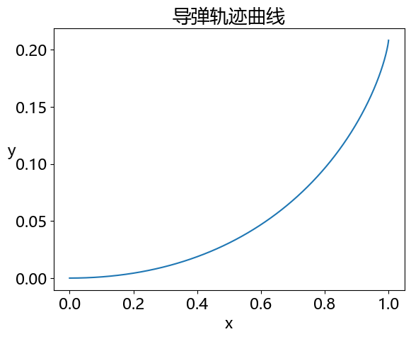
例8.8（序例8.2）二阶常微分方程的数值解（方程8.10）

$\begin{cases} (1-x)\frac{d^2y}{dx^2} = \frac{1}{5} \sqrt{1+\frac{dy}{dx}^2}, 0 < x \leq 1 \\ y(0) = 0, y'(0) = 0 \end{cases}$

解：鉴于Python只能求解一阶常微分方程的数值解，因此对于高阶微分方程必须先化简为一阶方程进行求解。对以上公式引入 $y_1 = y, y_2 =y'$ 则方程可转化为如下异界微分方程组：

$\begin{cases} y_1' = y_2 &, y_1(0) = 0 \\ y_2' = \frac{1}{5(1-x)} \sqrt{1+y_2^2} &, y_2(0) = 0 \\ \end{cases}$

对以上方程组进行python编程可得：

# Lec0406: 例8.8 二阶常微分方程的数值解
from scipy.integrate import odeint
import numpy as np
import matplotlib.pyplot as plt
plt.rcParams['font.sans-serif'] = ['Microsoft YaHei']  # 使用微软雅黑字体显示标签

dy = lambda y,x: [y[1], np.sqrt(1+y[1]**2)/5/(1-x)]   # 定义方程组y[0]=y1, y[1]=y2
x0 = np.arange(0, 1, 0.00001)                         # 定义x的初值
y0 = odeint(dy, [0, 0], x0)                           # 使用odeint求解数值解
plt.plot(x0, y0[:,0])
plt.xlabel('x')
plt.ylabel('y', rotation=True)
plt.title('导弹轨迹曲线')
plt.show()

例8.9 Lorenz模型的混沌效应

# Lec0407: 例8.9 Lorenz 模型的混沌效应
from scipy.integrate import odeint
import numpy as np
import pylab as plt
plt.rcParams['font.sans-serif'] = ['Microsoft YaHei']  # 使用微软雅黑字体显示标签


# 1. 定义模型函数
np.random.seed(2)                # 为了比较的稳定性，将随机数种子固定
sigma, rho, beta = (10, 28, 8/3)
# 此处使用序列f[0-2]表示公式中的x, y, z, 即状态变量
model = lambda x, t: [sigma*(x[1]-x[0]), rho*x[0]-x[1]-x[0]*x[2], x[0]*x[1]-beta*x[2]]    # 定义匿名微分方程组

# 2. 生成初值t0，并求解初值的数值解
t0 = np.linspace(0, 50, 5000)
x01 = np.random.rand(3)   #初始值
res1 = odeint(model, x01, t0)   #求数值解

plt.figure(figsize=(14,4))
plt.subplots_adjust(wspace=0.6)
ax1= plt.subplot(131, projection='3d')
ax1.plot(res1[:,0], res1[:,1], res1[:,2], 'r')         # 画轨线
ax1.set_xlabel('x')
ax1.set_ylabel('y')
ax1.set_zlabel('z')
ax1.set_title('Lorenz模型1')

# 3. 生成第二组初值，给定一个很小的变化量0.000001，并求解新初值的数值解
x02 = x01 + 0.000001
res2 = odeint(model, x02, t0)  # 初值变化后，再求数值解
ax2= plt.subplot(132, projection='3d')
ax2.plot(res2[:,0], res2[:,1], res2[:,2], 'r')         # 画轨线
ax2.set_xlabel('x')
ax2.set_ylabel('y')
ax2.set_zlabel('z')
ax2.set_title('Lorenz模型2(\delta = 0.000001)')

# 4. 计算两组初值的距离
ax3= plt.subplot(133)
ax3.plot(t0, res1[:,0] - res2[:,0], '.-')              #画x(t)的差
ax3.set_xlabel('t')
ax3.set_ylabel('M1-M2', rotation=True)
ax3.set_title('Lorenz模型混沌效应')
plt.show()

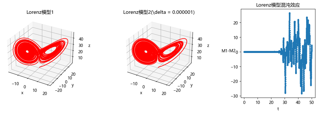
【结果分析】从结果来看，虽然初值之间只有细微的变化 $\delta = 0.000001$ ，但随着时间的推进，两组数值解的轨迹偏差越来越大，呈现出明显的混沌效应。

例8.10 一个慢跑者在平面上按如下规律跑步

$X = 10 + 20 \cos t, Y = 20 + 15 \sin t \tag{8.10.1}$

突然有一只狗攻击他，这只狗从原点出发，以恒定速率 $w$ 跑向慢跑者，狗运动方向始终指向慢跑者。分别求出 $w=20, w=5$ 时，狗的运动轨迹。

相关解答请参考：【案例07】慢跑者追逐问题

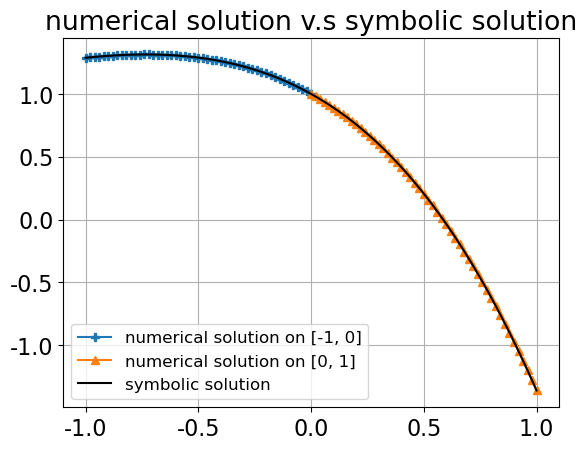
例8.11 求解二阶线性微分方程 $y'' - 2y' + y = e^x, y(0)=1, y'(0)=-1$ ，在区间 [-1, 1] 上的数值解，并与符号解进行比较。

问题分析：
求数值解时，由于 odeint 只能处理一个未知数，因此首先需要做变量替换使用数组变量 $t$ 表示 $y$ 和 $y'$ ，设 $t = [t_1, t_2] = [y, y']$ ，则二阶微分方程可化成如下的一阶微分方程组：

$\begin{cases} t_1' = t_2, & t_1(0) = 1 \\ t_2' = 2t_2 - t_1 + e^x, & t_2(0) = -1 \end{cases}$

在以上的微分方程中， $t_1(0)=1, t_2(0)=-1$ 表示初值，因此我们可以将原来的定义域 $[-1, 1]$ 划分为 $[0, 1]$ 以及 $[0, -1]$ 两个区域，分别求解数值解。

虽然理论上，数值求解方法（如odeint）可以处理包含0点的连续区间，但在某些情况下，特别是在处理具有奇异点、突变点或数值不稳定性的微分方程时，将区间分割成几部分可能会得到更好的结果。

以下是，计算微分方程符号解与数值解的代码。

# Lec0409: 例8.11 二阶线性微分方程的数值解
from scipy.integrate import odeint
import numpy as np
import sympy as sp
import matplotlib.pyplot as plt
plt.rc('axes', unicode_minus=False)   # 解决保存图像时负号'-'显示乱码问题

# 1. 数值解
# 1.1 计算数值解（以0点为分隔，分段计算数值解）
dt = lambda t, x: [t[1], 2*t[1] - t[0] + np.exp(x)]    # 定义微分方程
x1 = np.linspace(0, -1, 20)                    # 生成 [0,-1]的插值区间
s1 = odeint(dt, [1, -1], x1)                   # 求解数值解主函数
x2 = np.linspace(0, 1, 20)                     # 生成 [0,1]的插值区间
s2 = odeint(dt, [1, -1], x2)                   # 求解数值解主函数
# 1.2 绘制数值解曲线
plt.plot(x1, s1[:,0], 'P-', label='numerical solution on [-1, 0]')   # 绘制[0,1]上的数值解 
plt.plot(x2, s2[:,0], '^-', label='numerical solution on [0, 1]')    # 绘制[-1,0]上的数值解

# 2. 符号解
# 2.1 计算符号解
sp.var('x'); 
y = sp.Function('y')
eq = y(x).diff(x,2)-2*y(x).diff(x)+y(x)-sp.exp(x)   # 定义微分方程
con = {y(0):1,y(x).diff(x).subs(x,0):-1}      # 定义微分方程的初值
s = sp.dsolve(eq, ics=con)                    # 求解符号解主函数
sx = sp.lambdify(x, s.args[1], 'numpy')       # 转换成匿名函数，其中arg[0]为函数名，arg[1]为函数表达式
x3 = np.linspace(-1, 1, 100);                 # 生成 [-1,1]的插值区间
s3 = sx(x3)                                   # 基于解析解求解数值解
# 2.2 绘制符号解曲线
plt.plot(x3, s3, 'k-', label='symbolic solution')
plt.title('numerical solution v.s symbolic solution')
plt.legend()
plt.grid(True)
plt.show()

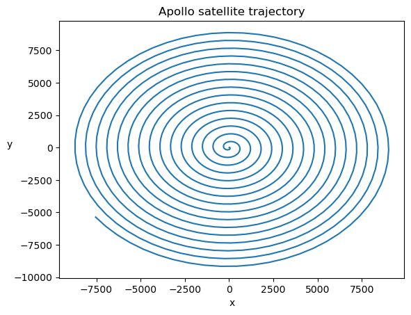
例8.12 已知阿波罗卫星的运动轨迹 (x, y) 满足如下方程：

$\begin{cases} \frac{d^2 x}{dt^2} = 2\frac{dy}{dt} + x - \frac{\lambda(x + \mu)}{r^3_1} - \frac{\mu(x -\lambda)}{r^3_2} \\\\ \frac{d^2 y}{dt^2} = -2\frac{dx}{dt} + y - \frac{\lambda y}{r^3_1} - \frac{\mu y}{r^3_2} \end{cases}$

其中 $\mu = 1/82.45, \lambda = 1-\mu, r_1 = \sqrt{(x+\mu)^2 + y^2}, r_2 = \sqrt{(x+\lambda)^2 + y^2}$ 。设存在初值 $x(0)=1.2, x'(0)=0, y(0)=0, y'(0)=-1.0494$ ，试求阿波罗卫星的运动轨迹，并绘制出该轨迹图。

将微分方程中的变量替换为 $z=[z_0,z_1, z_2, z_3]$ ，其中 $z_0 = x, z_1 = \frac{dx}{dt}, z_2=y, z_3=\frac{dy}{dt}$ ，则原二阶微分方程组可化为如下一阶方程形式：

$\begin{cases} \frac{dz_0}{dt} = z_1, & z_0(0) = 1.2 \\ \frac{dz_1}{dt} = 2z_3 + z_0 - \frac{\lambda(z_0 + \mu)}{((z_0 + \mu)^2 + z_2^2)^{3/2}} - \frac{\mu(z_0 - \lambda)}{((z_0 + \lambda)^2 + z_2^2)^{3/2}}, & z_1(0) = 0 \\ \frac{dz_2}{dt} = z_3, & z_2(0) = 0 \\ \frac{dz_3}{dt} = -2z_1 + z_2 - \frac{\lambda z_2}{((z_0 + \mu)^2 + z_2^2)^{3/2}} - \frac{\mu z_2}{((z_0 + \lambda)^2 + z_2^2)^{3/2}}, & z_3(0) = -1.0494 \end{cases}$

根据以上方程组，编写Python程序求解阿波罗卫星的运动轨迹如下：

# Lec0410: 例8.12 阿波罗卫星的运动轨迹
from scipy.integrate import odeint
import numpy as np
import pylab as plt

# 1. 定义超参数常数值
mu = 1/82.45
lamda = 1-mu

# 2. 定义微分方程dz: dz_1/dt, dz_2/dt, dz_3/dt, dz_4/dt
dz = lambda z, t: [z[1], 
                2*z[3]+z[0]-lamda*(z[0]+mu)/((z[0]+mu)**2+z[2]**2)**(3/2)-mu*(z[0]-lamda)/((z[0]+lamda)**2+z[2]**2)**(3/2), 
                z[3],
                -2*z[1]+z[2]-lamda*z[2]/((z[0]+mu)**2+z[2]**2)**(3/2)-mu*z[2]/((z[0]+lamda)**2+z[2]**2)**(3/2)]

# 3. 求解微分方程
t = np.linspace(0, 100, 1001)                 # 定义自变量t的插值区间
res = odeint(dz, [1.2, 0, 0, -1.0494], t)     # 求解微分方程

# 4. 绘制运动轨迹
plt.plot(res[:, 0], res[:, 2])    # plt.plot(x, y) 表示绘制二维曲线
plt.xlabel('x')
plt.ylabel('y', rotation=0)
plt.title('Apollo satellite trajectory')
plt.show()

例8.13 利用表8.1给出的近两个世纪的美国人口统计数据（以百万为单位），建立人口预测模型，最后用它预报2010年美国的人口。

# Lec0411: 例8.13 美国人口预测模型
import numpy as np
import pandas as pd
from scipy.optimize import curve_fit

# 1. 数据预处理
data = pd.read_excel('../Data/Lec04/data8_13.xlsx', header=None)      # 使用Pandas读取xlsx数据
data = data.values                                                    # 将pandas数据转换为numpy数组
data_population = data[1::2,:]                                        # 将第1,3,5行数据存入变量x中，即从第1行开始，以间隔2读取数据，直到最后一行。
data_population = data_population[~np.isnan(data_population)]         # 提出有效数据，去掉数据中值为nan的元素
data_year = np.linspace(1790, 2000, 22)                               # 生成年份序列，也可从数据中读取
# data_year = data[1::2,:]                                            # 将第1,3,5行数据存入变量x中，即从第1行开始，以间隔2读取数据，直到最后一行。
# data_year = data_year[~np.isnan(data_year)]                         # 提出有效数据，去掉数据中值为nan的元素，此处应注意和人口数据对齐
x0 = data_population[0]
t0 = data_year[0]
year_pred = 2010

# 2. 方法一：非线性最小二乘估计(公式8.32)
x = lambda t, r, x_max: x_max/(1+(x_max/x0-1)*np.exp(-r*(t-t0)))        # 设人口数量为 x 简历Logistic人口增长模型（原模型的解）
bd = [(0, 100), (0.1,1000)]                                             # 约束参数人口出生率r和最大人口数的下界和上界
coef1 = curve_fit(x, data_year[1:], data_population[1:], bounds=bd)[0]  # 常微分方程建模方法参数
r = coef1[0]
x_max = coef1[1]
pred1 = x(year_pred, r, x_max)
print('方法一：非线性最小二乘估计')
print('人口增长率为：{:.4f}， 最大人口为：{:.2f} 百万'.format(coef1[0], coef1[1]))
print('2010年的预测值为：{:.4f} 百万'.format(pred1))

# 3. 方法二：线性最小二乘估计-前向差分(8.34)
delta_t = 10
n = len(data_population)
b1 = np.diff(data_population)/delta_t/data_population[:-1]  #构造常数项列
a1 = np.vstack([np.ones(n-1), -data_population[:-1]]).T
coef2 = np.linalg.pinv(a1) @ b1
r = coef2[0]
x_max = r/coef2[1]
pred2 = x(year_pred, r, x_max)
print('-----------------------------------')
print('方法二：线性最小二乘估计-前向差分')
print('人口增长率为：{:.4f}， 最大人口为：{:.2f} 百万'.format(r, x_max))
print('2010年的预测值为：{:.4f} 百万'.format(pred2))

# 3. 方法三：线性最小二乘估计-后向差分(8.35)
b2 = np.diff(data_population)/delta_t/data_population[1:]  #构造常数项列
a2 = np.vstack([np.ones(n-1), -data_population[1:]]).T
coef3 = np.linalg.pinv(a2) @ b2
r = coef3[0]
x_max = r/coef3[1]
pred3 = x(year_pred, r, x_max)
print('-----------------------------------')
print('方法三：线性最小二乘估计-后向差分')
print('人口增长率为：{:.4f}， 最大人口为：{:.2f} 百万'.format(r, x_max))
print('2010年的预测值为：{:.4f} 百万'.format(pred3))

方法一：非线性最小二乘估计
人口增长率为：0.0274， 最大人口为：342.44 百万
2010年的预测值为：282.6799 百万
-----------------------------------
方法二：线性最小二乘估计-前向差分
人口增长率为：0.0325， 最大人口为：294.39 百万
2010年的预测值为：277.9634 百万
-----------------------------------
方法三：线性最小二乘估计-后向差分
人口增长率为：0.0247， 最大人口为：373.51 百万
2010年的预测值为：264.9119 百万

例8.14 捕食者-被捕食者方程组

# Lec0412: 例8.14 捕食者与被捕食者
import numpy as np

# 1. 数据准备
t0 = np.array([0,1,2,3,4,5,6,8,10,12,14,16,18])
x0 = np.array([60,63,64,63,61,58,53,44,39,38,41,46,53])
y0 = np.array([30,34,38,44,50,55,58,56,47,38,30,27,26])

# 2. 构造差分方程组
dt = np.diff(t0)   # 计算t的差分
dx = np.diff(x0)   # 计算x的差分
dy = np.diff(y0)   # 计算y的差分
equ1 = np.vstack([x0[:-1], -x0[:-1]*y0[:-1], np.zeros((2,12))]).T    # 方程1的系数 
equ2 = np.vstack([np.zeros((2,12)), -y0[:-1], x0[:-1]*y0[:-1]]).T    # 方程2的系数
equs = np.vstack([equ1, equ2])                      # 构造线性方程组系数矩阵（公式8.37右边）
Y = np.hstack([dx/dt, dy/dt])                       # 构造线性方程组常数项列（公式8.37左边）

# 3. 使用最小二乘方法拟合系数
coef = np.linalg.pinv(equs)@Y                         # 线性最小二乘法
print('参数 a, b, c, d 的值分别为:', coef)

参数 a, b, c, d 的值分别为: [0.19073636 0.00482605 0.48288662 0.00953575]

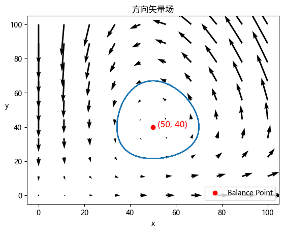
例8.15 捕食者-被捕食者方程组（续8.14）

# Lec0413: 例8.15 捕食者与被捕食者（续）

import numpy as np
import sympy as sp
import matplotlib.pylab as plt
from scipy.integrate import odeint
plt.rcParams['text.usetex'] = False
plt.rcParams['font.sans-serif'] = ['Microsoft YaHei']

# 1. 求微分方程的解，获取物种的稳定点
sp.var('x,y')
eq = [0.2*x - 0.005*x*y, -0.5*y + 0.01*x*y]
res = sp.solve(eq, [x,y])
print(' 方程的解一: {}；\n 方程的解二: {}'.format(res[0], res[1]))

# 2. 绘制方向矢量场
# 2.1 绘制方向矢量场图
x = np.linspace(0,100,10)
x, y = np.meshgrid(x,x)
u = 0.2*x - 0.005*x*y         # 方向分量u
v = -0.5*y + 0.01*x*y         # 方向分量v 
plt.quiver(x, y, u, v)
plt.xlabel('x')
plt.ylabel('y', rotation=0)
plt.title('方向矢量场')
plt.plot(res[1][0], res[1][1], 'ro', label='Balance Point')
text_BP = '(' + str(int(res[1][0])) + ', ' + str(int(res[1][1])) + ')'
plt.text(res[1][0]+2, res[1][1], text_BP, fontsize=12, color='red')
plt.legend(loc='lower right')

# 2.2 求解常微分方程的数值解
def func(f, t):               # 构造微分方程组，也可使用lambda匿名函数进行定义
    x, y = f
    return [0.2*x-0.005*x*y, -0.5*y+0.01*x*y]

t = np.linspace(0, 100, 1000) # 定义月份自变量t的插值区间
s = odeint(func, [70, 40], t) # 求解常微分方程的数值积分。func: 积分函数，[70, 40] 初始条件，t 时间自变量

# 2.3 根据数值解获取 x, y的取值范围，并可视化到矢量场中
x_min = min(s[:,0])
x_max = max(s[:,0])
print('x 的取值范围：[{}, {}]'.format(x_min, x_max))
y_max = max(s[:,1])
y_min = min(s[:,1])
print('y 的取值范围：[{}, {}]'.format(y_min, y_max))
plt.plot(s[:,0], s[:,1]);
plt.show()

方程的解一: (0.0, 0.0)；
方程的解二: (50.0000000000000, 40.0000000000000)
x 的取值范围：[34.22924234120125, 70.0]
y 的取值范围：[21.47710791964677, 66.96332841715827]

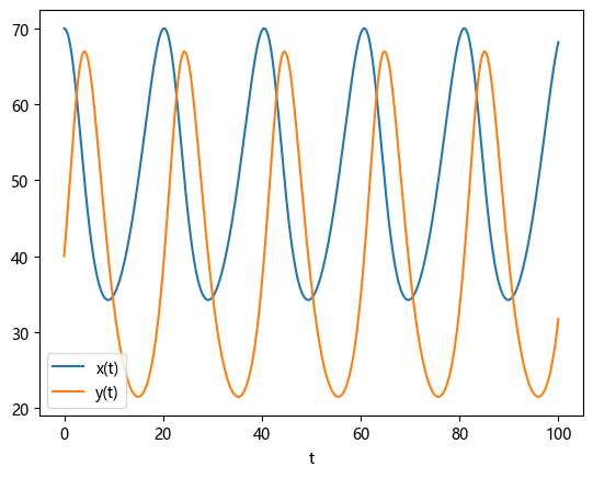
# 3. 绘制兔子x(t)和狐狸y(t) 种群数量变化曲线
import matplotlib
matplotlib.use('TkAgg')

plt.figure()
plt.plot(t, s[:,0], label='x(t)')
plt.plot(t, s[:,1], label='y(t)')
plt.legend()
plt.xlabel('t')

# 以下代码可以通过交互方式计算增长或减少的周期（需要取消TkAgg GUI接口的注释）
print(">>> 请点击x(t)或y(t)解曲线上相邻的极小点（注意确保两个点的纵轴相等，即种群数量相等）!")
x = plt.ginput(2)
print('点击的点', x)
T = x[1][0] - x[0][0]
print("周期T为: ", T)

请点击x(t)或y(t)解曲线上相邻的极小点（注意确保两个点的纵轴相等，即种群数量相等）!
点击的点 [(75.7258064516129, 21.534873267361476), (55.32258064516129, 21.534873267361476)]
周期T为:  -20.40322580645161

二、差分方程

例8.16 贷款问题

# Lec0414: 例8.16 贷款问题

# 1. 定义初始变量
Q = 300000                                  # 贷款总额
annual_rate = 0.051                         # 年利率
monthly_rate = annual_rate / 12             # 月利率
loan_term_years = 30                        # 贷款期限
loan_term_months = loan_term_years * 12     # 贷款期限（月）

# 2. 基于解析法求解每月还款额（根据解析解进行代入计算）
monthly_payment = (1+monthly_rate)**loan_term_months*Q*monthly_rate/((1+monthly_rate)**loan_term_months-1)
print('（解析法）每月应还款金额为: {:.2f} 元'.format(monthly_payment))

# 3. 使用等额本息还款标准公式计算每月还款额
monthly_payment = Q * (monthly_rate / (1 - (1 + monthly_rate)**(-loan_term_months)))
print(f'（公式法）每月应还款金额为: {monthly_payment:.2f} 元')

（解析法）每月应还款金额为: 1628.85 元
（公式法）每月应还款金额为: 1628.85 元

例8.17（续例8.13）再论美国人口增长模型

# Lec0415: 例8.17 再论美国人口增长模型
import numpy as np
import pandas as pd

# 1. 数据预处理
data = pd.read_excel('../Data/Lec04/data8_13.xlsx', header=None)      # 使用Pandas读取xlsx数据
data = data.values                                                    # 将pandas数据转换为numpy数组
data_population = data[1::2,:]                                        # 将第1,3,5行数据存入变量x中，即从第1行开始，以间隔2读取数据，直到最后一行。
data_population = data_population[~np.isnan(data_population)]         # 提出有效数据，去掉数据中值为nan的元素

A = np.vstack([data_population[:-1], data_population[:-1]**2]).T      # 系数矩阵 x_k, x_k^2 
coef = np.linalg.pinv(A) @ data_population[1:]                        # 使用常微分方程建模方法参数
pred = coef[0]*data_population[-1] + coef[1]*data_population[-1]**2   # 输出预测值
print('alpha = {:.4f}, beta = {:.4f}'.format(coef[0], coef[1]))
print('2010年人口预测值为: {:.4f} 百万'.format(pred))

alpha = 1.2095, beta = -0.0004
2010年人口预测值为: 307.6809 百万

【第04讲】微分方程的求解 返回首页